This is just some fluff. After all this time looking at the industry-funded clinical trials [RCTs], I’ve learned a few tricks for spotting the mechanics of deceit being used, but I realize that I need to say a bit about the basic science of RCTs before attempting to catalog things to look for. Data Transparency is likely coming, but very slowly. And even with the data, it takes a while to reanalyze suspicious studies – so to these more indirect methods. I expect there will be a few more of these posts along the way – coming mostly on cold rainy week-end days like today when there’s not much else going on. If you’re not a numbers type, just skip this post. But if you’re someone who wants to contribute to the methodology of vetting these RCTs, email me at 1boringoldman@gmail.com. Examples appreciated. It’s something any critical reader needs to know how to do these days…
The word sta·tis·tics is derived from the word state, originally referring to the affairs of state. With usage, it has come to mean general facts about a group or collection and the techniques used to compare groups. In statistical testing, we assume groups are not different [the null hypothesis], then calculate the probability of that assumption. If it’s less than some value called alpha [0.05], we reject the null hypothesis and assume the groups are significantly different.
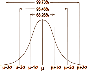 In statistical testing, assumptions abound. For continuous variables, we assume that the data follow a normal distribution, so we can simplify the dataset into just three numbers: the mean [μ], the standard deviation [σ], and the number of subjects [n]. In an RCT, with just those numbers for the placebo group and the drug group, we can calculate the needed probability. In the normal distribution, all the items between two standard deviations on either side of the mean make up 95% of the sample. Values outside those limits make up only 5% of the sample. In doing statistical testing for the difference between two groups [assuming for the moment an equal σ and n], when the probability of the null hypothesis is 0.05 or less [p < 0.05], we feel confident that the groups are significantly different. But that only tells us that the groups are different – not how different.
 In this simple two group example, calculating the p value depends on having the means [μ1 and μ2], the standard deviations [σ1 and σ2], and the two sample sizes [n1 and n2]. And this is about as far as they got in my medical school version of a statistics course in the dark ages called the 60s
  [only scratching the surface of the field]. So those of us doing research had to add some other degrees. They do a better teaching job in these modern times [with computers to do the heavy number crunching instead of the calculators that shook the table and sounded like Gatling guns]. And with the increased computer power came much more sophisticated statistical testing allowing the evaluation of many more factors in the models.
This is a case where one wonders if the technological advances have been all that helpful. In the past, medications were evaluated on clinical grounds. The efficacy scale was simple. It had it doesn’t work, it sometimes works, and it works – a scale suited to an effective medications. With the modern clinical trials, much smaller differences are the rule – sometimes in the range of absurdity. So, as most people know in the abstract, a p < 0.05 doesn’t necessarily denote clinical significance. It may mean absolutely nothing or conversely something of real value. But in spite of that knowledge, our eyes are invariably drawn to the ubiquitous p value like a magnet.
One attempt to get at a more relevant index of efficacy is to standardize the magnitude of the difference between the means of the two samples in some way – for example Cohen’s d [a way to compute the strength of the effect]. It’s the difference in the means expressed as a percent of the pooled standard deviation. Back to assuming an equal σ and n in the two groups, it would be:
d = (μ1 – μ2) ÷ σ
While there’s no strong standard for d like there is for p, the general gist of things is that: d = 0.250 [25%] is weak, d = 0.50 [50%] is moderate, and d = 0.75 [75%] is strong. Note: for groups of unequal size or distribution, the pooled σ is:

This graphic makes this point better, and gets around to why I’m writing this:

 Even a strong Cohen’s d isn’t a huge separation – plenty of overlap still in the picture. So when you’re looking at Effect Sizes, don’t think it looks like the figure on the left [d = 4]. You’re usually still back in the land of sometimes when you’re looking at these Effect Sizes in a Clinical Trial report in a journal article.
Another point. You may have noticed that you need μ, σ, and n to calculate statistical significance, but only μ and σ to calculate Cohen’s d. The strength of effect is independent of the sample size. You can figure out how these thing relate to each other. With a drug that has a moderate effect [eg d = 0.50] you need only a small sample size to achieve statistical significance [even less if it’s strong]. But with a weak effect [d = 0.250], you need to have a whole lot more subjects in your study. Again, assuming two groups with equal size and distribution, the relationship looks like this:
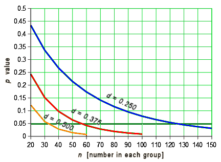
While these are the nuts and bolts of how one does Power Analysis when planning a clinical trial to figure out the needed sample size, that’s not why this graph is here. Most RCTs have p values listed, but many don’t have any version of the Effect Size [Cohen’s d, Odds Ratio, NNT, etc], probably because they’re weak sisters. So one thing to look for is that they have very large sample sizes. It’s in order to get that magic p < 0.05 they’re looking for to legitimize a weak effect. When the Effect Size is missing, you often have enough information to calculate it using the formulas above. Note: It’s common to have the Standard Error [se or sem] rather than the Standard Deviation [sd or σ]. But it’s easily converted using the formula:
se = σ ÷ √n or σ = se × √n
A common way to get those large samples is by having many sites with small numbers from each [from all over the world]. That introduces another covariate [number of sites], so it’s important to see if SITE is included in the statistical model and testing. But more about that part next time there’s a cold and rainy lost weekend…


 O! be some other name:
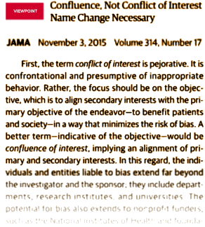
 While there was, indeed, a lot of corruption in the years around the turn of the century, to dismiss it with something tanamount to "but there was a lot of that going around" as if it were a fad or a pesky virus hardly rises to any reasonable medical or academic standard. It’s an argument as lame as "… such policies might restrain innovation and delay translation of basic discoveries to clinical benefit." Medicine arose in ancient history and survived for centuries not based on powerful scientific advances. Those advances are only in their second century. Medicine prevailed because it was among the few professions that was able to adhere to a consistent and enduring ethical stance. A resistance to outside Conflicts of Interest has been an implied element of that ethic throughout our history. Arguments such as those expressed in this JAMA viewpoint article simply have no place in our tradition or our literature. And to have these recent articles actually advocating for conflicted authorship in our two major journals [NEJM:
  While I’ve given up political blogging for good, there is a story I followed in the past that may finally be coming to a long awaited resolution. It’s the story of Burma [Myanmar] which is under a military dictatorship backed by the world’s largest standing army. Since my summary in 2007 [
 In statistical testing, assumptions abound. For continuous variables, we assume that the data follow a normal distribution, so we can simplify the dataset into just three numbers: the mean [μ], the standard deviation [σ], and the number of subjects [n]. In an RCT, with just those numbers for the placebo group and the drug group, we can calculate the needed probability. In the normal distribution, all the items between two standard deviations on either side of the mean make up 95% of the sample. Values outside those limits make up only 5% of the sample. In doing statistical testing for the difference between two groups [assuming for the moment an equal σ and n], when the probability of the null hypothesis is 0.05 or less [p < 0.05], we feel confident that the groups are significantly different. But that only tells us that the groups are different – not how different.
  In this simple two group example, calculating the p value depends on having the means [μ1 and μ2], the standard deviations [σ1 and σ2], and the two sample sizes [n1 and n2]. And this is about as far as they got in my medical school version of a statistics course in the dark ages called the 60s
  [only scratching the surface of the field]. So those of us doing research had to add some other degrees. They do a better teaching job in these modern times [with computers to do the heavy number crunching instead of the calculators that shook the table and sounded like Gatling guns]. And with the increased computer power came much more sophisticated statistical testing allowing the evaluation of many more factors in the models.
 Even a strong Cohen’s d isn’t a huge separation – plenty of overlap still in the picture. So when you’re looking at Effect Sizes, don’t think it looks like the figure on the left [d = 4]. You’re usually still back in the land of sometimes when you’re looking at these Effect Sizes in a Clinical Trial report in a journal article.

 dramatic decrease in capillary density. That was a significant finding, but hardly the point of the study – an observation along the way. The classic example is the discovery of Penicillin. Alexander Fleming, a veteran of WWI, was involved in looking for antimicrobial agents, having seen so much sepsis in that war. He sure wasn’t studying dirty petri dishes. But when he saw a bacteria-free ring around a mold in a dirty petri dish, he knew what he was looking at – an observation along the way.
![Clinical Neuroscience timeline [2005] Clinical Neuroscience timeline [2005]](http://1boringoldman.com/images/insel-1.gif)
 It just doesn’t seem to register anymore that this class of articles reporting clinical trials is published in academic journals, but it has no real connection to anything "academic." I’ve referred to the authors highlighted in red as "tickets," as if their function is to certify admission to the journals. I recently suggested facetiously in